NCAA Volleyball Survey
Summary of the findings from the NCAA D1 Women's Indoor Volleyball Strength and Conditioning Coaches Survey.


In this post, I'll be describing the steps behind the methodology of how I gathered, and analyzed the results from the NCAA D1 Indoor Women's Volleyball survey.
Distribution of the Survey
As all of us know, in the wake of the COVID-19 pandemic response, the NCAA has suspended countable athletic-related activities and participation through the spring 2020 semester. While summer access is still unknown, many athletic departments, medical staffs, and strength and conditioning professionals are focused on identifying the necessary preparatory time for "successful" women's indoor volleyball competitive participation (defined as the beginning of 20-hour CARA weeks).
I'm Adam Ringler, Assistant Director of Sports Performance at University of Colorado. I'm leading this research project both to (1) share evidence with our Colorado administration and medical team and (2) to distribute the collected results through this email and strength and conditioning news mediums.
My hopes are to collect, compare, and share cohort consensus regarding the necessary strength and conditioning preparatory time needed for "successful" Division 1 NCAA women's indoor volleyball competitive participation.
The linked survey focuses on leveraging your professional expertise and opinions surrounding the necessary strength and conditioning time allocations. The survey is only 5 questions and takes less than 15 seconds. No personal identifiable information is collected and all responses are anonymous outside of conference affiliation.
https://cuboulder.qualtrics.com/jfe/form/SV_5gVFLh2HFaJwoC1
Assessment of the Responses
One of the first steps was making sure that the appropriate packages are installed in the notebook. pandas, matplotlib, and seaborn does most of the heavy lifting.
# Importing relevant packages with their alias
import pandas as pd
import matplotlib.pyplot as plt
import matplotlib
import seaborn as sns
Next will be creating the initial data set from the exported CSV file provided by the Qualtrics website.
# Read data
url = "https://raw.githubusercontent.com/AdamRingler/NCAAdata/master/NCAA.csv"
ncaa = pd.read_csv(url,index_col=0)
I performed some simple cleaning of the data set, where I dropped out the values that were incomplete in the survey and then also created a dataframe that specifically subsetted responses from PAC-12 schools.
ncaa_removestring = ncaa.iloc[2:]
ncaa_removenan=ncaa_removestring.dropna()
ncaa_clean = ncaa_removenan
ncaa_pac12 = ncaa_removenan[ncaa_removenan['Q1'] == 'Pac-12']
Many of the remaining code snippets are rather repetitive but I thought I would include them to increase transparency behind the data and visualizations.
# Set initial plot options
sns.set_style('white')
plt.figure(figsize = (28, 8))
# Create a countplot
sns.countplot(x = 'Q1',
data = ncaa_clean,
palette = ['lightgreen'], alpha = 0.6)
# Despine visualizations
sns.despine()
# Final styling
plt.ylabel('Number of responses', fontsize = 12, fontweight = 'semibold')
plt.xlabel('Division 1 Conferences', fontsize = 12, fontweight = 'semibold')
plt.title('Participating Conferences in Survey', fontsize = 20, fontweight = 'semibold')
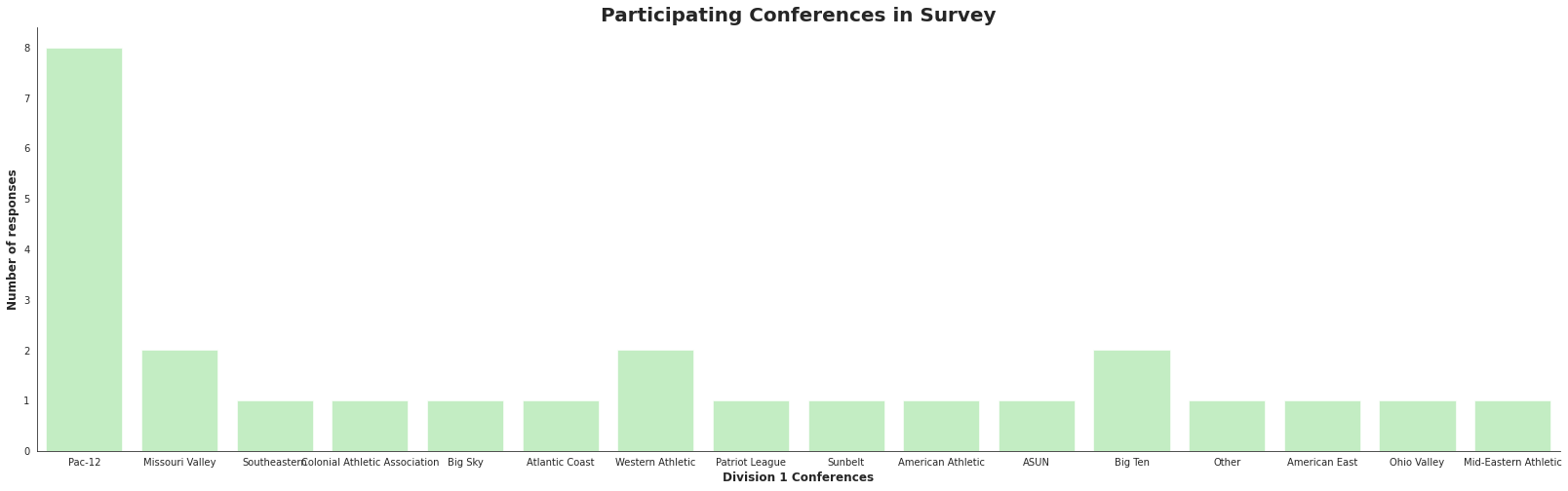
plt.show()Two ways of looking at essentially the responses from the survey, below being a bar chart of a count of participating conferences and the second figure representing a table.
# Create Table
conferences = ncaa_clean.groupby('Q1')
conferences['Q1'].count().sort_values(ascending=False)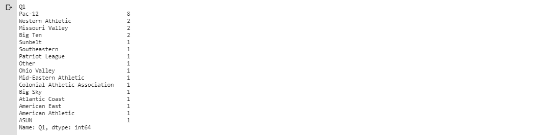
# Set initial plot options
sns.set_style('white')
plt.figure(figsize = (12, 8))
# Create a countplot
sns.countplot(x = 'Q2',
data = ncaa_clean,
order = ['1 Week', '2 Weeks', '3 Weeks', "4 Weeks", "5 Weeks", '6 Weeks', '7 Weeks', '8+ Weeks'],
palette = ['skyblue'], alpha = 0.6)
# Despine visualizations
sns.despine()
# Final styling
plt.ylabel('Number of responses', fontsize = 12, fontweight = 'semibold')
plt.xlabel('Weeks of training', fontsize = 12, fontweight = 'semibold')
plt.title('Minimum Weeks of S&C for NCAA Volleyball', fontsize = 14, fontweight = 'semibold')
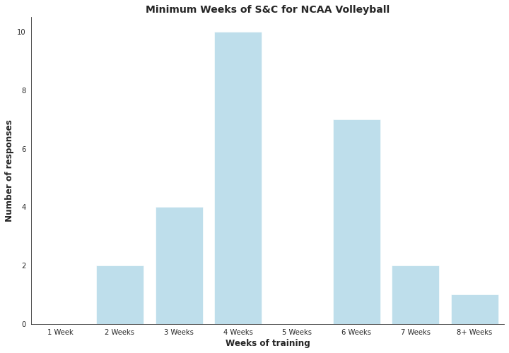
plt.show()What is captured is that the resounding thought across all conferences is that the minimum amount of time necessary to prepare women's indoor volleyball athletes to be ready for the start of in-season training is 4 weeks, followed by 6 weeks.
# Set initial plot options
sns.set_style('white')
plt.figure(figsize = (12, 8))
# Create a countplot
sns.countplot(x = 'Q3',
data = ncaa_clean,
order = ['1 Week', '2 Weeks', '3 Weeks', "4 Weeks", "5 Weeks", '6 Weeks', '7 Weeks', '8+ Weeks'],
palette = ['skyblue'], alpha = 0.6)
# Despine visualizations
sns.despine()
# Final styling
plt.ylabel('Number of responses', fontsize = 12, fontweight = 'semibold')
plt.xlabel('Weeks of training', fontsize = 12, fontweight = 'semibold')
plt.title('Preferred Weeks of S&C for NCAA Volleyball', fontsize = 14, fontweight = 'semibold')
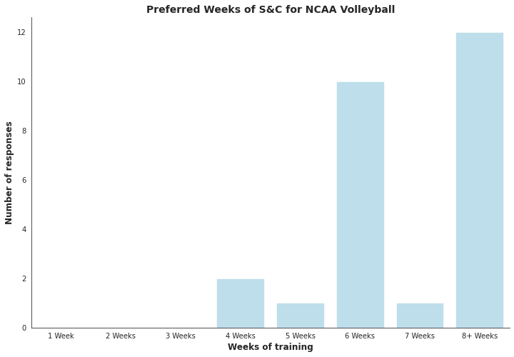
plt.show()However, when strength & conditioning professionals are asked about the optimal and preferred time allocation they feel would most appropriately allow them to prepare athletes for the start of season, most strength and conditioning coaches would prefer to have 8+ weeks to prepare their athletes.
# Set initial plot options
sns.set_style('white')
plt.figure(figsize = (12, 8))
# Create a countplot
sns.countplot(x = 'Q4',
data = ncaa_clean,
order = ['1/Week', '2/Week', '3/Week', "4/Week", "5/Week", '6/Week', '7/Week', '8+/Week'],
palette = ['skyblue'], alpha = 0.6)
# Despine visualizations
sns.despine()
# Final styling
plt.ylabel('Number of responses', fontsize = 12, fontweight = 'semibold')
plt.xlabel('Training sessions', fontsize = 12, fontweight = 'semibold')
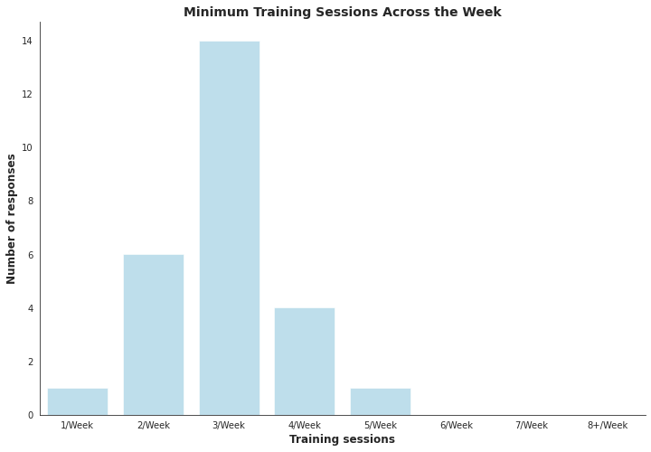
plt.title('Minimum Training Sessions Across the Week', fontsize = 14, fontweight = 'semibold')
plt.show()When asked about the minimum number of training sessions required to prepare the athletes for the start of 2020 season, strength and conditioning coaches reported a minimum of 3 sessions a week.
# Set initial plot options
sns.set_style('white')
plt.figure(figsize = (12, 8))
# Create a countplot
sns.countplot(x = 'Q5',
data = ncaa_clean,
order = ['1/Week', '2/Week', '3/Week', "4/Week", "5/Week", '6/Week', '7/Week', '8+/Week'],
palette = ['skyblue'], alpha = 0.6)
# Despine visualizations
sns.despine()
# Final styling
plt.ylabel('Number of responses', fontsize = 12, fontweight = 'semibold')
plt.xlabel('Training sessions', fontsize = 12, fontweight = 'semibold')
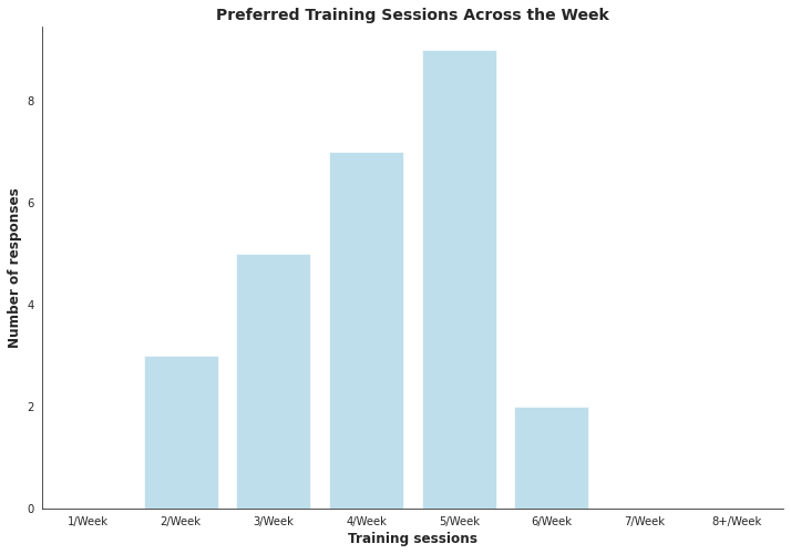
plt.title('Preferred Training Sessions Across the Week', fontsize = 14, fontweight = 'semibold')
plt.show()When asked about the optimal and preferred allocation of training sessions per week, a number of training sessions required to prepare the athletes for the start of 2020 season, strength and conditioning coaches reported a preference of 5 sessions a week.
# Set initial plot options
sns.set_style('white')
plt.figure(figsize = (12, 8))
# Create a countplot
sns.countplot(x = 'Q2',
data = ncaa_pac12,
order = ['1 Week', '2 Weeks', '3 Weeks', "4 Weeks", "5 Weeks", '6 Weeks', '7 Weeks', '8+ Weeks'],
palette = ['mediumpurple'], alpha = 0.6)
# Despine visualizations
sns.despine()
# Final styling
plt.ylabel('Number of responses', fontsize = 12, fontweight = 'semibold')
plt.xlabel('Weeks of training', fontsize = 12, fontweight = 'semibold')
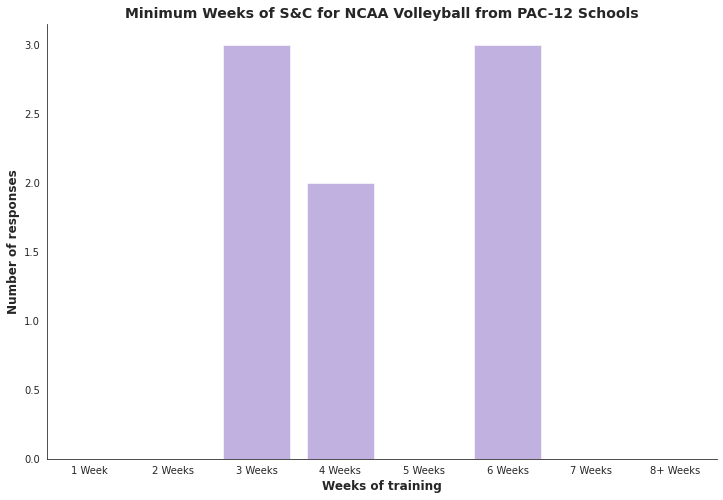
plt.title('Minimum Weeks of S&C for NCAA Volleyball from PAC-12 Schools', fontsize = 14, fontweight = 'semibold')
plt.show()A PAC-12 Analysis of Responses
The remainder of the visualizations are examining the PAC-12 responses. Indicated in the figure alone, the minimum number of weeks that PAC-12 Strength & Conditioning coaches felt was necessary to prepare women's indoor volleyball athletes to be ready for the start of in-season training responded is distributed across 3 weeks and 6 weeks.
# Set initial plot options
sns.set_style('white')
plt.figure(figsize = (12, 8))
# Create a countplot
sns.countplot(x = 'Q3',
data = ncaa_pac12,
order = ['1 Week', '2 Weeks', '3 Weeks', "4 Weeks", "5 Weeks", '6 Weeks', '7 Weeks', '8+ Weeks'],
palette = ['mediumpurple'], alpha = 0.6)
# Despine visualizations
sns.despine()
# Final styling
plt.ylabel('Number of responses', fontsize = 12, fontweight = 'semibold')
plt.xlabel('Weeks of training', fontsize = 12, fontweight = 'semibold')
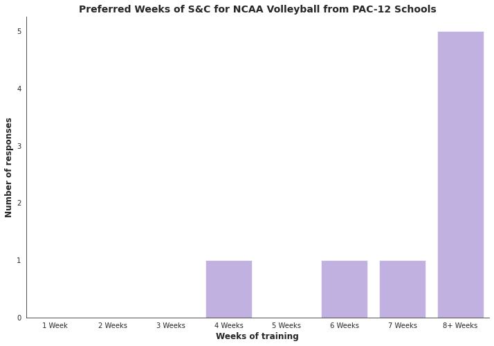
plt.title('Preferred Weeks of S&C for NCAA Volleyball from PAC-12 Schools', fontsize = 14, fontweight = 'semibold')
plt.show()When PAC-12 strength & conditioning professionals were asked about the optimal and preferred time allocation they feel would most appropriately allow them to prepare athletes for the start of season, PAC-12 strength and conditioning coaches overwhelmingly reported that would prefer to have 8+ weeks to prepare their athletes.
# Set initial plot options
sns.set_style('white')
plt.figure(figsize = (12, 8))
# Create a countplot
sns.countplot(x = 'Q4',
data = ncaa_pac12,
order = ['1/Week', '2/Week', '3/Week', "4/Week", "5/Week", '6/Week', '7/Week', '8+/Week'],
palette = ['mediumpurple'], alpha = 0.6)
# Despine visualizations
sns.despine()
# Final styling
plt.ylabel('Number of responses', fontsize = 12, fontweight = 'semibold')
plt.xlabel('Training sessions', fontsize = 12, fontweight = 'semibold')
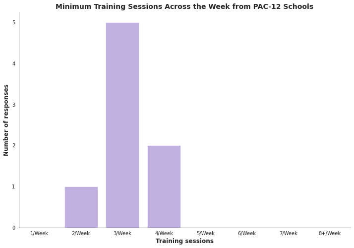
plt.title('Minimum Training Sessions Across the Week from PAC-12 Schools', fontsize = 14, fontweight = 'semibold')
plt.show()When asked about the minimum number of training sessions required to prepare the athletes for the start of 2020 season, PAC-12 strength and conditioning coaches reported a minimum of 3 sessions a week.
# Set initial plot options
sns.set_style('white')
plt.figure(figsize = (12, 8))
# Create a countplot
sns.countplot(x = 'Q5',
data = ncaa_pac12,
order = ['1/Week', '2/Week', '3/Week', "4/Week", "5/Week", '6/Week', '7/Week', '8+/Week'],
palette = ['mediumpurple'], alpha = 0.6)
# Despine visualizations
sns.despine()
# Final styling
plt.ylabel('Number of responses', fontsize = 12, fontweight = 'semibold')
plt.xlabel('Training sessions', fontsize = 12, fontweight = 'semibold')
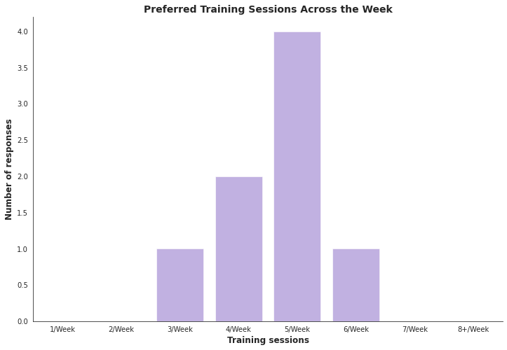
plt.title('Preferred Training Sessions Across the Week', fontsize = 14, fontweight = 'semibold')
plt.show()When asked about the optimal and preferred allocation of training sessions per week, a number of training sessions required to prepare the athletes for the start of 2020 season, PAC-12 strength and conditioning coaches reported a preference of 5 sessions a week.
Raw Data Set
 AdamRingler
Conclusion
As a wrap-up to this survey and Python data project, what the data suggests is that polled strength and conditioning professionals indicated a time minimum of 4 weeks in order to prepare their women indoor volleyball athletes. The polled PAC-12 strength and conditioning professionals are split between 3 weeks and 6 weeks. There is an agreement among conferences for a preference of 8+ weeks of dedicated strength and conditioning work prior to the begin of fall season.
The results also indicate consensus among conferences and professionals that the minimum amount of training sessions per week would be 3 sessions per week, with a shared preference of having a 5 sessions per week.